Five scheduling experiments, one stubborn baseline

Five attempts at per-sample interventions, the mechanism each one tripped on, and why uniform sampling kept winning.

Not all training examples are equally useful to a model, which makes it tempting to train more efficiently by spending more of the model's attention on the valuable ones — sampling them more often, or weighting them more heavily — rather than treating every example the same. This post is about whether that intuition holds up in practice.

Uniform sampling turned out to be a difficult baseline to beat.

I didn't expect that. I expected that better per-sample information would translate into better training schedules. Instead I ended up running five increasingly sophisticated interventions that all landed within touching distance of the same baseline. The interesting part wasn't that they failed. It was that each failure ruled out one explanation for the previous one — until the pattern of failure itself became the result.

I ended up testing three hypotheses, each one in response to the previous one's failure:

• that a good warmup estimate of per-sample value would remain useful throughout training,
• then, that the scores were simply becoming stale and needed refreshing,
• and finally, that if no version of scheduling could move the baseline, weighting gradients directly might.

Each one was, in hindsight, the natural next thing to try. The first hypothesis was tested with a single intervention; the second and third with two variants each, for five experiments in total. None of them held up. By the end I was left looking at the pattern itself, not at any of the explanations I'd brought into the work.

Setup

I tested across two text classification benchmarks: DBpedia 14 (30,000 examples per seed) and AG News (22,000 examples per seed). The training model was DistilBERT — random-init for DBpedia, pretrained for AG News — for 25 and 10 epochs respectively. The asymmetry isn't arbitrary: pretrained DistilBERT saturates DBpedia within 2–3 epochs, leaving no convergence curve for a scheduler to act on; random-init gives 25 epochs of genuine learning. AG News is small enough that random-init would underfit, so the pretrained start is the sensible operating point there. Per-sample scores were computed from a separate pretrained DistilBERT used in inference-only mode, then fed into whichever scheduler the experiment was testing.

Each intervention was compared against uniform-sampling baseline on the same locked criteria: higher average validation accuracy across the run, faster to target accuracy on every seed tested, and final accuracy no more than 1 percentage point below baseline. An intervention had to pass all three to count as beating uniform. None did.

Worth flagging: the experiments aren't all on equal footing. The first hypothesis was tested most rigorously — two seeds, two datasets, multiple hyperparameter variants. The second and third were tested at one seed on DBpedia each. By the time I got to the more elaborate interventions, the failure pattern from the simpler case was already pointing in a consistent direction, and the question I cared about was whether different mechanisms produced the same failure.

What if the warmup scores stay useful?

This was the starting belief: a good warmup pass produces a per-sample value estimate, and that estimate should be useful for the rest of training. The most natural way to act on it is also the simplest. Bias sampling toward high-scoring examples early when the model is learning fast, then anneal toward uniform later as the model converges. A small floor keeps low-scoring examples in rotation so nothing gets dropped entirely. Two control knobs: how steep the initial bias is, and at what point in training the anneal toward uniform begins. The structural pieces follow the patterns I'd been reading about in the curriculum learning and importance sampling literature.

Across both datasets and both seeds, the static scheduler underperformed uniform on AUC across all four runs — but only DBpedia seed 11 showed more than a marginal gap (−0.66pp); the other three landed between −0.04 and −0.17pp, with AG News seed 17 even running above uniform in the final epochs before netting slightly negative.

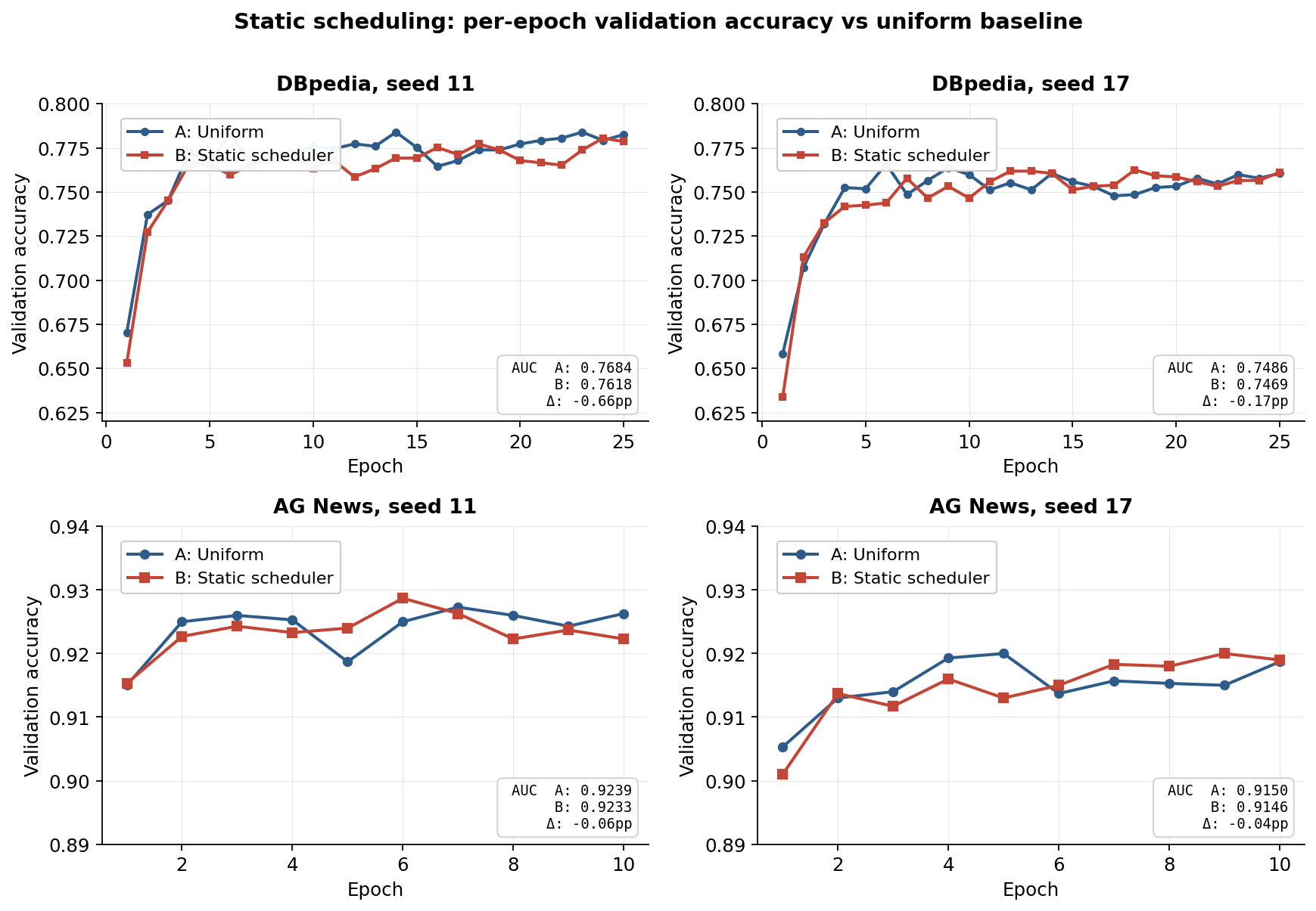
The two curves stay entangled for the whole run. Where the early bias was supposed to buy a head start, the scheduler if anything begins slightly behind — on both DBpedia seeds it sits below uniform at epoch 1 before the gap closes. From there neither side holds an edge for long: the curves cross and recross within a band that looks like seed-to-seed wobble rather than a scheduler doing work. What never appears is a sustained, directional advantage — no stretch where the early bias or the later anneal opens a gap and keeps it. The trajectories end where uniform ends, by a path that runs alongside it the whole way.

The warmup score isn't necessarily wrong. It's frozen. It captures the model's view at one point in training, while the model itself keeps changing. A sample that looks redundant at warmup based on geometric similarity in embedding space may later define a decision boundary; another that looks highly informative early may become uninteresting once the model has absorbed it. The score doesn't track any of this — it captures the warmup-model's state, not the trajectory of states the training model will pass through.

If that mechanism is the failure mode, the fix is obvious. Don't commit at warmup. Update the scores during training so they reflect the model's current state. That's the next attempt.

What if the scores simply go stale?

The second hypothesis: warmup scores aren't enough, but updated scores would be. I tested two versions, differing only in which signal got rescored.

The first used an informativeness score: a function of per-sample loss and prediction margin, designed to be high for examples the model is still uncertain about. The second used entropy of the predicted class distribution as the signal — another member of the informativeness/uncertainty family, but computed directly from the output distribution rather than from loss and margin. High entropy means the model's confidence is spread across classes; low entropy means it's confident about one. I'll refer to these as G0 and G2 — the labels they had in the experimental record, useful as shorthand when comparing across charts later.

Both used the same shard-based refresh structure, which is worth describing briefly because the results depend on it. The training pool is split into three shards. Training begins with two epochs of uniform sampling — a warmup that gives the model some initial competence before any rescoring is attempted. After that, every five epochs, one shard takes its turn being rescored: the current model runs over those examples in inference mode and produces a fresh score for each one (informativeness for G0, entropy for G2). Those new scores then update the sampling weights for the next five-epoch window. Higher-scored examples — those the current model is least confident about — get sampled more often, the same mild-bias mechanism as the static case but with weights that refresh as the model learns. The rotation continues for as long as training runs: on DBpedia's 25 epochs, five refreshes at epochs 3, 8, 13, 18, and 23. The intent is a schedule that keeps adapting to what's still hard — never frozen at the warmup snapshot.

On DBpedia, both versions underperformed uniform on AUC — G0 by about 0.2pp, G2 by about 0.6pp. These are single-seed observations, not error-barred estimates, but the direction was consistent and neither version reached target accuracy faster than uniform at any tested checkpoint. By the locked criteria, both were fails.

The interesting part is what happens to the rescoring signal itself during training.

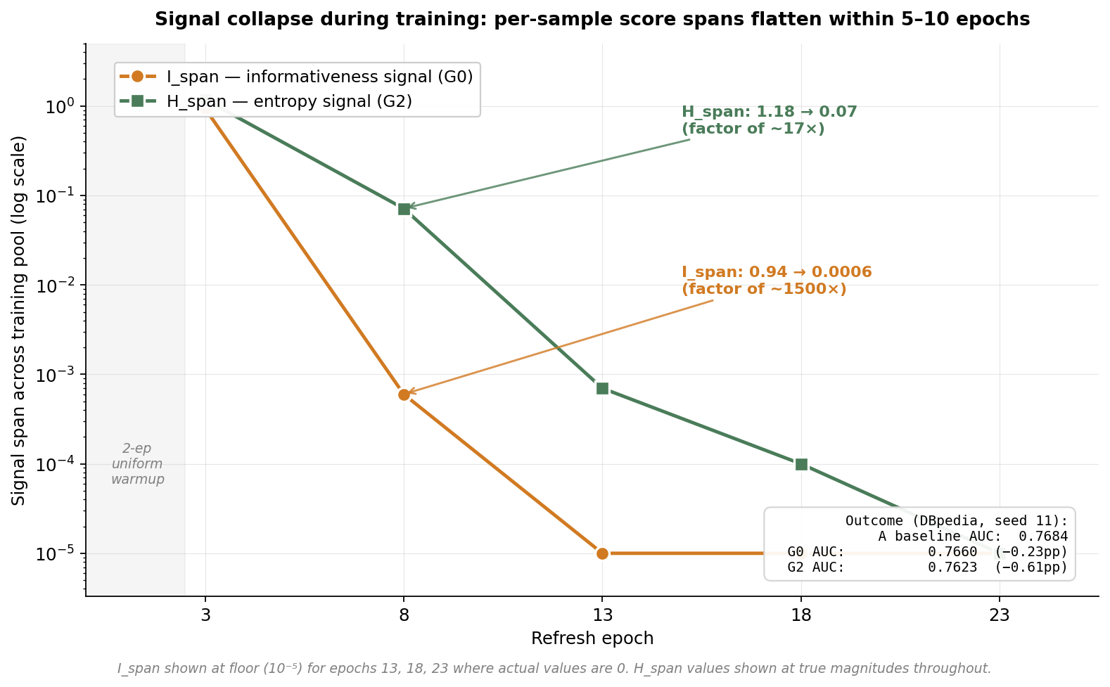
At the first refresh — epoch 3, right after the two-epoch warmup — the informativeness signal spans 0.94 across the training pool: most-informative and least-informative examples are clearly distinct, and the score is doing its job. Five epochs later the span has collapsed to 0.0006, and by the third refresh it's effectively zero. The entropy signal follows the same path more slowly — 1.18 down to 0.07 and still falling — until it too reaches the floor.

What's happening: as training progresses, the model becomes confident about most of the training pool. The informativeness signal flattens because the per-sample losses are all small. The entropy signal flattens because the model's predictions concentrate on a single class for almost every example. After the first refresh window, the rescoring is operating on a signal that no longer distinguishes samples from one another. The "dynamic" scheduler is dynamic in name only; what it's actually doing is updating weights from a flat distribution to a slightly different flat distribution.

That this happens in both signals — informativeness and entropy, which capture different things — rules out a particular kind of objection. It would be reasonable to say "you picked the wrong signal; try a different one." The fact that two structurally different signals both collapse on the same timescale suggests the problem isn't with the choice of signal. It's with the assumption underneath all signals of this kind: that informativeness or uncertainty over the training pool stays distinguishable long enough for a rescoring schedule to act on it. By the time the schedule has data to act on, the model has already moved past the regime where the signal carries information.

If staleness was the problem in the first hypothesis, signal collapse is the problem in the second. The natural follow-up: maybe the issue isn't scheduling at all. Maybe sampling-based interventions are the wrong mechanism, and a more direct intervention — scaling each sample's contribution to the gradient — would work where scheduling didn't.

What if sampling is the wrong intervention altogether?

By this point I had run through the scheduling variants worth trying. Before concluding the approach was dead, I tried the cruder instrument: skip sampling entirely and reach inside the gradient step. Instead of using per-sample scores to decide which samples appear in a batch, use them to decide how much each sample contributes to the loss within a batch. Every sample still gets seen in normal proportion; high-value samples just get their loss multiplied by a higher weight before the gradient step.

I tested two strengths, labeled G3 and G4 in the experimental record. G3 used a mild weighting (α=0.20) that scales loss multipliers in a narrow range around 1.0. G4 used an aggressive weighting in the [0.5, 2.0] range — meaning the most-weighted samples contribute four times as much per-batch as the least-weighted ones. In both cases, the per-sample weighted losses are averaged across the batch before the gradient step. If gradient-level intervention works at all, the aggressive version should produce a larger effect than the mild one.

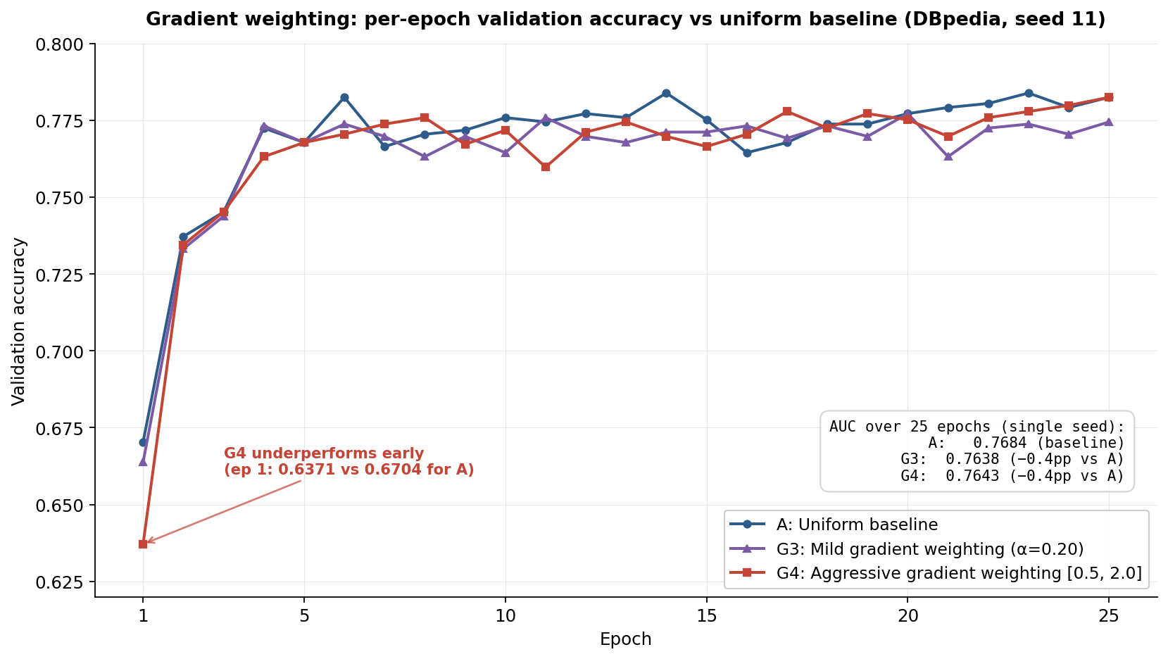
Both fail. G3 and G4 each underperform uniform by about 0.4pp on AUC, and G4's nominal edge of about 0.05pp over G3 is well inside single-seed run-to-run wobble — not a real difference. The load-bearing observation is that scaling the weighting strength up several times over didn't change the outcome: if aggressive weighting were amplifying a useful signal, the two should look different, and they don't. The plausible reading, given that the entropy signal driving this weighting is the same one that collapsed in the previous hypothesis, is that there isn't much signal left to amplify by the time training is well underway.

Since each batch is just a small sample of the training pool, the within-batch spread of entropies can't exceed the pool-level spread that collapsed in Chart 2 — so by the same epochs, individual batches are working with nearly-flat entropies too.

That changes what the weighting actually does inside a batch. With per-sample entropies all close to each other, multiplying the loss by entropy-derived weights effectively scales every example by something close to the same number. The "weighted" loss is weighting one nearly-flat distribution against another. Scaling a flat signal more aggressively doesn't make it less flat.

What this means

Three hypotheses, all falsified — and each one in a way that points at the same underlying observation: the model's current state determines what each sample contributes, and that state changes faster than any per-sample valuation can track. Static commits before knowing. Dynamic chases a collapsing signal. Gradient amplifies a flat one. By the time the model had learned enough for rescoring to become informative, the scores themselves had largely flattened. None of the falsifications opened up a direction that worked.

This isn't an argument from first principles that scheduling can't work. It's a report of what happened under fixed verdict criteria, on two benchmarks, with the score families I had — a different model, dataset, or signal could in principle produce a different outcome. What the experiments establish is a consistent boundary at the scale I tested, not a theoretical impossibility.

After five attempts, what surprised me wasn't that the interventions failed. It was how consistently the simplest baseline survived them. The more sophisticated the intervention became, the more stubborn the baseline looked. The interventions weren't unreasonable — they were exactly the things I expected to work — but optimization appears more robust to per-sample manipulation than I expected.

Methodology footnote: All experiments used DistilBERT — random-init for DBpedia, pretrained for AG News — at max sequence length 12 (DBpedia) and 128 (AG News). Intervention parameters: static scheduler used bias exponent η=1.5, anneal transition at 40% of training, and an ε=0.05 floor on per-sample weights; dynamic rescoring used a two-epoch warmup then refresh every five epochs over three rotating shards; gradient weighting used per-batch entropy-based loss scaling, mild (α=0.20) and aggressive ([0.5, 2.0]). Full methodology available on request.

This is part of an ongoing series of notes on ML training dynamics.