The operating envelope of data pruning: what holds, and what breaks

Notes from a multi-dataset NLP study on how aggressively training data can be trimmed before accuracy starts to slip.

Anyone who's trained a model at production scale has done some version of the math: GPU-hours times dollars per hour times how many runs you'll need. After enough runs, the inefficiency becomes hard not to notice. And a fair amount of that compute goes into near-duplicates, samples the model has effectively learned, and samples that don't seem to change what the model learns regardless of how long you train.

In earlier work I built a small library of per-sample signals to score training data — redundancy, informativeness, prediction stability. When I tried using them to control training in pursuit of better accuracy, none of the interventions worked: good descriptors, bad control levers.

This post takes a different question. If the signals can't make training better, can they make it more efficient? Specifically: if a redundancy score accurately identifies samples that overlap with others, can we remove those samples and train on less data while preserving accuracy?

The short answer turns out to be: yes, within bounds. Below I'll show what those bounds look like.

Setup

I tested redundancy-based pruning on three NLP classification benchmarks: IMDB (sentiment, 2-class), AG News (news topic, 4-class), and Yahoo Answers (topic, 10-class). The model is a DistilBERT classifier in all cases, trained on a single A100 GPU. For each dataset I ran a short warmup pass to establish embeddings, scored every training sample by how redundant it is with the rest of the dataset, using nearest-neighbor distance in embedding space, then trained the full model on the surviving data after removing the top-scoring (most redundant) fraction.

I varied three things: how long to warm up (5%, 15%, or 25% of training epochs), how much to prune (10%, 20%, or 30%), and the random seed (two seeds per condition). That's a small grid — 3 datasets × 3 warmup fractions × 3 pruning rates × 2 seeds, 54 runs in total — and the conclusions need to be read as drawn from that grid, not from an exhaustive sweep. These were deliberately modest-scale runs — the goal was to probe how the signal behaves, not to chase peak accuracy.

A note on selector choice: across the envelope charts (the heatmap and the 25%-warmup chart), each dataset uses the selector best matched to its structure — the global selector for the balanced datasets (IMDB and AG News), and the class-stratified selector for the imbalanced one (Yahoo Answers). The class-stratified selector was the targeted fix for an imbalanced-data failure mode I'll explain in the class-balance section below. The envelope charts therefore show each dataset under its appropriate selector, not under a single uniform choice.

What works at 10%

Across every warmup fraction tested, 10% pruning landed within 1 percentage point of the full-data baseline on average across datasets. The best condition — 15% warmup, 10% pruning — came in at −0.12pp.

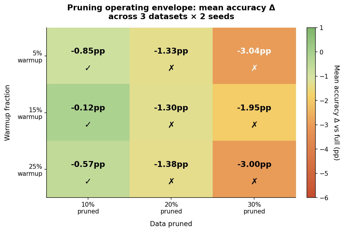
Mean accuracy change relative to a full-data baseline, averaged across IMDB, AG News, and Yahoo Answers (two seeds each). ✓ indicates the condition is within 1 percentage point of the full baseline; ✗ indicates it exceeds 1pp. At 10% pruning, every warmup condition stayed within 1pp on average. The 15% warmup / 10% pruning condition — at −0.12pp — was the strongest result tested.

The warmup is the first portion of the same training run, not a separate pass: I run the model on full data through warmup, score and prune, then continue training on the surviving subset. For 25% warmup and 10% pruning that's about 92.5% of full-data compute — a ~7.5% single-run saving on training, before accounting for the cost of the scoring pass itself (a forward pass plus nearest-neighbor distances over the full dataset). That overhead eats into the single-run figure but amortizes across repeated runs that reuse the scores (sweeps, retrains, replicates), at which point the saving grows toward the full 10%.

10% pruning holds across all three task structures — binary sentiment, four-class news, and ten-class topical Q&A — with one caveat: Yahoo Answers, the imbalanced dataset, sits closest to the line and crosses it at the highest warmup. The redundancy score is identifying samples that add very little new information, broadly across these different task structures. Why imbalance changes the picture is the subject of the next section.

What breaks at 20% and beyond

The picture changes when you push harder. At 20% pruning, no warmup condition averages within 1pp. At 30%, the drop is larger — three of three warmup conditions land between −1.95pp and −3.04pp on average. The warmup effect itself isn't clean across this grid: at 30% pruning, 15% warmup (−1.95pp) actually beats 25% warmup (−3.00pp) by over a point — non-monotonicity two seeds can't fully resolve.

The aggregate also hides per-dataset variation worth looking at. Here's the longest warmup condition (25% — the one with the most full-data scoring behind it) broken out by dataset:

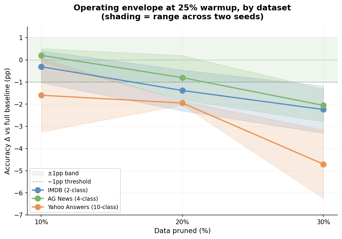
Per-dataset accuracy at the longest tested warmup condition (25% — the most full-data scoring), with shading showing the range across two seeds. AG News stays inside the band through 20% pruning; IMDB has crossed the −1pp threshold by 20%; Yahoo Answers, the imbalanced 10-class dataset, degrades faster. The aggregate heatmap above hides this variation. In practice, the safe pruning rate for a given dataset depends on its class structure, redundancy, and the accuracy tolerance of the use case.

On the two balanced datasets the slope is close to linear — steep enough that you cross a 1pp tolerance around 20%, where AG News's two seeds straddle the line and IMDB has already crossed it. Yahoo Answers behaves differently — already at −1.6 at 10%, with a real step down between 20% and 30%. At 30% pruning, all three datasets are clearly outside the safe zone.

This isn't the boundary of what the method can do. It's the boundary of what I tested. The point of these experiments was to test whether the signal supports meaningful pruning, not to discover the ceiling. The ceiling depends on the use case: a different model, different warmup, different datasets, different accuracy tolerance will push the envelope in either direction. What the data establishes is that signal-based pruning is real — where you set the operating point is a separate question.

The class-balance problem

There's a second finding that's specifically about imbalanced data, and it's worth pulling out because imbalance is the norm in real-world ML.

On Yahoo Answers (10 classes, with the most frequent class about 4× more common than the least), the naive pruning approach has a problem. The global selector ranks all samples by redundancy score and removes the top-scoring ones. But different classes have systematically different redundancy profiles — for reasons that come down to how internally similar each class's examples are — and the selector pulls hardest from the classes with the highest mean redundancy. The result is class-biased pruning. On this dataset the effect happens to track class size — smaller classes are hit harder, with Science & Math under-retained by 4.6pp. But the direct cause is the redundancy structure across classes, not the class sizes themselves.

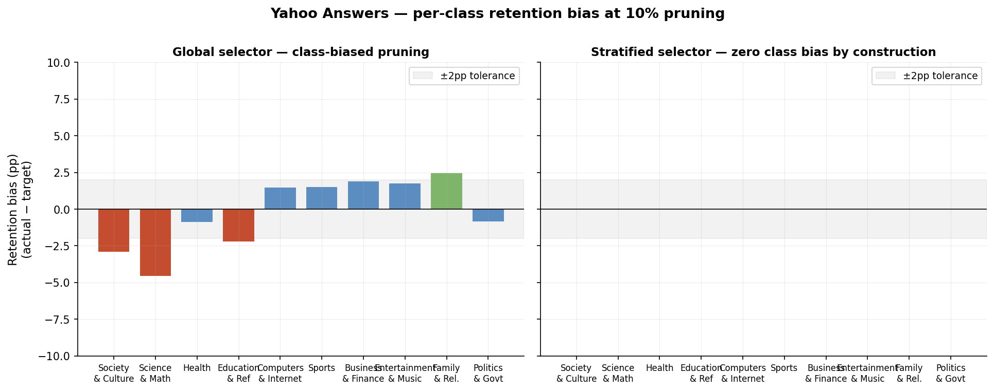
When the global selector ranks every sample by redundancy and removes the top-scoring ones, it pulls disproportionately from classes with higher mean redundancy — Science & Math is the worst-affected, retained 4.6pp below its proportional target. The stratified variant allocates the pruning budget within each class separately, so retention bias is zero by construction.

The fix is mechanical: allocate the pruning budget within each class separately, so 10% pruning means removing 10% of each class's samples, scored by within-class redundancy. The stratified selector has zero class-frequency bias by construction.

The end-task accuracy bears out the mechanical fix:

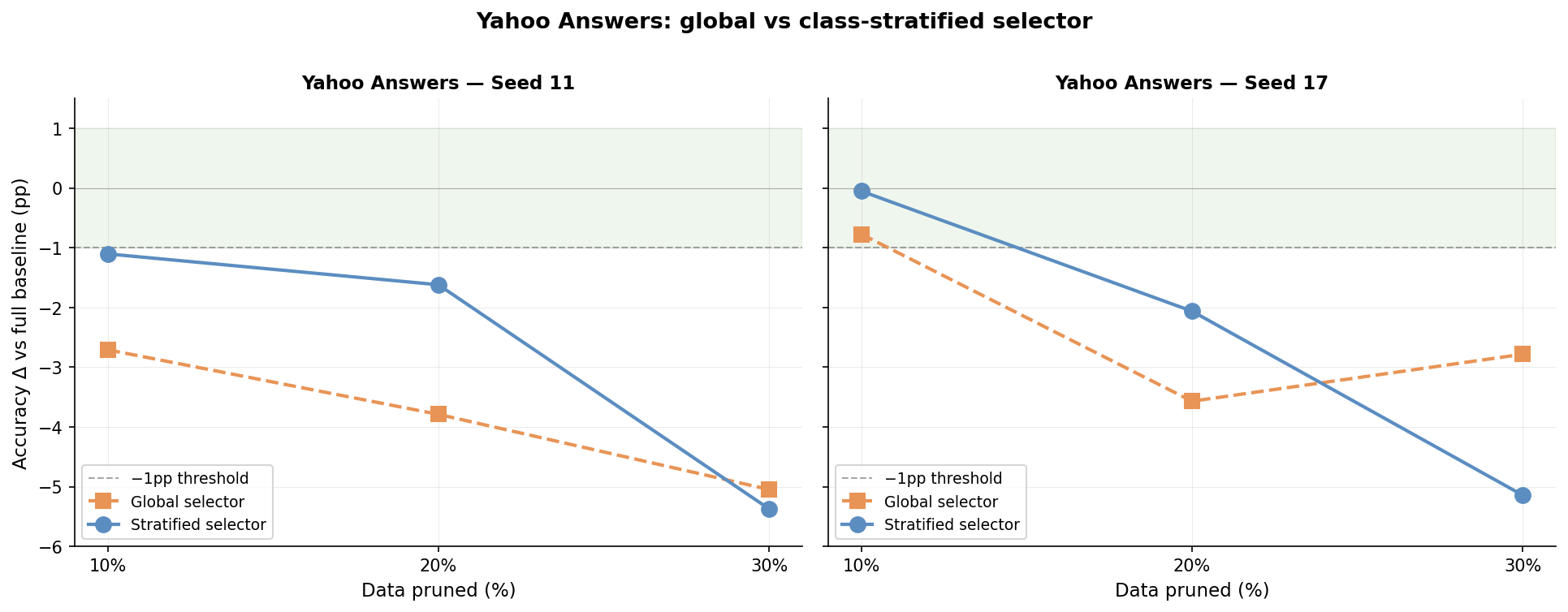
Test accuracy for the two selectors on Yahoo Answers at 10%, 20%, and 30% pruning, shown for both seeds at 10% warmup. The stratified selector outperforms the global one by 0.7-2.2pp at 10-20% pruning rates. At 30%, both approaches are well outside the safety band; the picture splits across seeds. The fix helps within the operating envelope; it doesn't extend it.

The stratified selector recovers about 0.7 to 2.2 percentage points at conservative pruning rates; the fix works within the operating envelope but doesn't extend it. At 30%, both approaches are well outside the safety band, and the picture splits across seeds: on seed 11 the two fail almost identically, while on seed 17 the stratified selector is meaningfully worse than the global one.

Seed 17 at 30% behaves oddly in a second way too: the global selector is non-monotonic across rates (−3.57pp at 20%, −2.78pp at 30%). Both observations plausibly trace to which specific samples each cut removed from the worst-affected classes — sample-level variance that two seeds can't fully resolve. The broader picture is unchanged: at 30%, neither approach preserves accuracy.

Worth noting: class-stratified sampling itself isn't novel — stratification is a well-established statistical technique. What the data shows is that signal-based redundancy selectors have a documented class-frequency bias on imbalanced data, and that the obvious stratification fix recovers most of the loss. Whether the bias has been characterized elsewhere in the data-pruning literature, I haven't dug into; the result holds either way.

What this means

The redundancy signal identifies samples accurately enough that removing the highest-scoring ones up to about 10% — and 20% in some dataset/warmup combinations — preserves accuracy within roughly a percentage point of full training. As noted earlier, the realized compute saving depends on warmup fraction and is restored toward the full 10% when scoring is amortized across multiple runs.

But "how aggressively can I prune" and "how much accuracy do I lose" don't trade off the same way across datasets. On the balanced datasets there's a roughly continuous tradeoff — accuracy falls at a near-constant slope — but the usable band is narrow: you leave a 1pp tolerance somewhere around 20%, and right at that line two seeds were already enough to land on either side. On the imbalanced dataset the relationship stops being smooth at aggressive rates. So the knob exists, but it's a narrow-range one on balanced data and an unstable one on imbalanced data at high pruning rates.

This matches the pattern from the earlier post on training dynamics. The signals are good descriptors of the training data — accurate enough that you can act on them and get real efficiency gains. But they're not a wide control dial — at best a narrow, dataset-dependent operating range. You can identify a conservative operating point that works, push past it cautiously, and accept that beyond a certain point the relationship becomes use-case-specific.

One thread I haven't taken up here: redundancy is one signal in a family. Informativeness and prediction-stability scores look at different properties — how much the model has yet to learn from each sample, and how robust its current prediction is to small perturbations. The post above is about removing data that's too similar to keep. A related question — separate from what's here — is whether the same kind of scoring could identify training data that's noisy or mislabeled, and what removing it would do. That's a different selector and a different study.

The honest framing: redundancy-based pruning works within bounds, and the bound is a decision the user makes based on their dataset and their accuracy tolerance. The contribution isn't a magic compression ratio. It's a tool that lets you make that decision with measured evidence.

Methodology footnote: Experiments used a DistilBERT classifier on IMDB, AG News, and Yahoo Answers, trained on a single A100 GPU, with two seeds and warmup fractions of 5% / 15% / 25%. Pruning rates of 10% / 20% / 30%. The 1pp accuracy threshold is a reference point, not a hard limit of the method. Full methodology details available on request.

This is part of an ongoing series of notes on ML training dynamics.